How to Make A Pie Chart in Excel

At the start of 2021, you were given the duty of creating a pie chart displaying which sort of material achieved the best performance on the Marketing Blog in 2020.

The topic was certainly significant, as it would affect the sort of material we created in 2021, as well as the identification of new chances for development. But, once you have gathered all pertinent data, you are stumped: how could you quickly make a pie chart to display your findings? Fortunately, we have worked it out for you.

Let's have a look at how to make a pie chart in excel for amazing marketing written reports. In addition, learn how to rotate a pie chart in Excel, burst a pie chart, and even construct a 3-dimensional version. When it comes to numbers, they don't hold much attention. But when your team visually sees the data, everything makes sense.

Pie charts are an excellent method to exhibit numerical data because they allow you to quickly compare the magnitude of different values while also making the full data set visible at a glance. And if you already have a column or row of data in an Excel file, you can create a pie chart in roughly five seconds.

This is how you do it:

How to Make A Pie Chart With Percentages in Excel

Pie charts, often known as circle graphs, are a common technique to demonstrate how much specific numbers or percentages contribute to the total. In such graphs, the full pie represents 100% of the total, while the pie slices indicate sections of the total. People adore pie charts, but visualisation experts despise them. You should know how to make a pie chart in excel.

The fundamental scientific reason for this is that the human eye is incapable of precisely comparing angles. Creating a pie chart in Excel is simple, requiring only a few button clicks. The essential element is to correctly arrange the source data in your worksheet and select the best pie chart type for your needs.

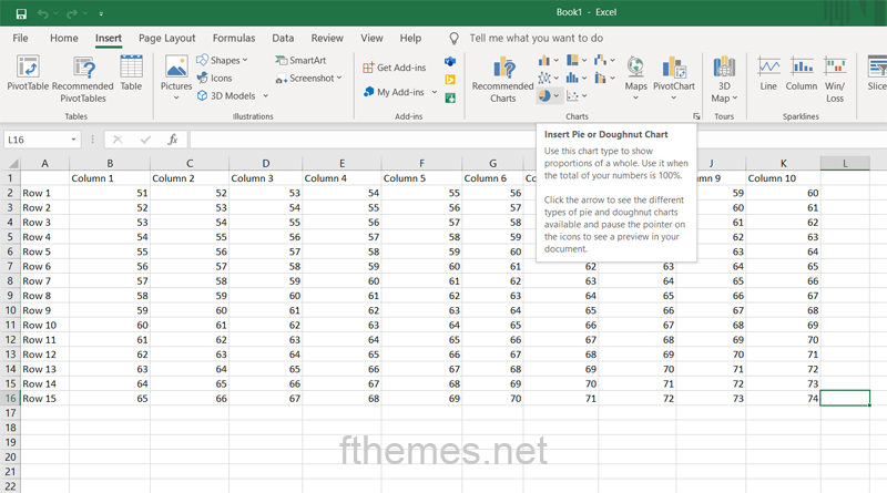
Step 1: First, you need to create a pie chart by preparing the data source for the pie chart.

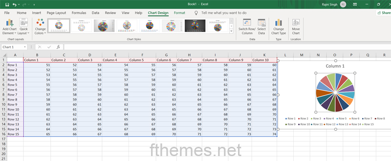
Step 2:  You need to go to the Insert tab and then make a choice between the chart type according to your preferences.

Step 3: This one is optional only if you wish to change the style of your pie chart then you need to pay a visit to the Insert button and then the Design tab and after that the charts group to try the different pie chart styles.

Step 4: Right-click on the slice of your pie chart after it gets added.

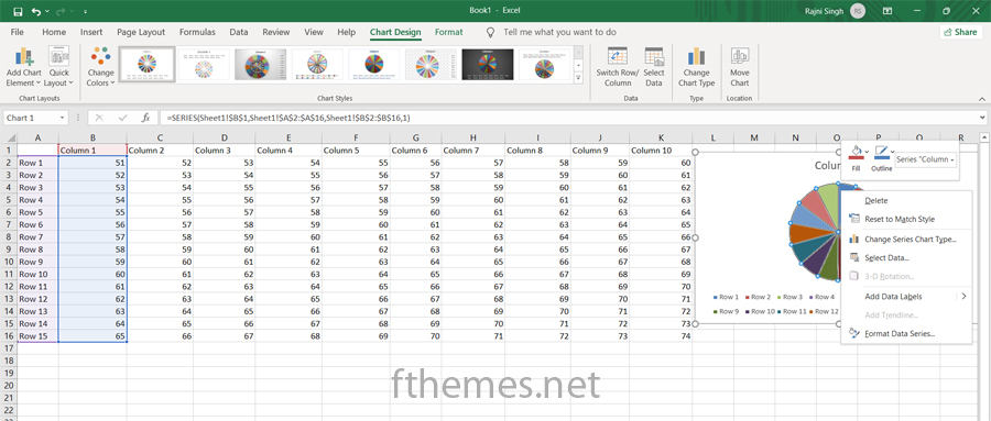
Step 5: Next just tap on the format data labels from the Context menu.

Step 6: On the format data labels, you need to select the values to be displayed in values or percentages.

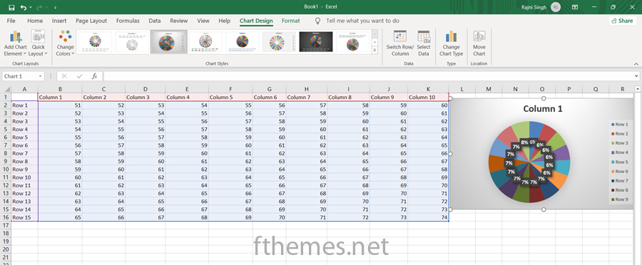
That's how easy it was!

How to Make A 3D Pie Chart in Microsoft Excel

If your Excel pie graph contains an excessive number of little slices, consider creating a Pie of Pie chart and displaying small slices on an extra pie that is a slice of the primary pie. The Bar of Pie graph is similar to the Pie of Pie graph in that the selected slices are presented on a secondary bar chart. Before all this, you should know how to make a pie chart in excel.

When you initiate making a pie chart in Excel, the final three data categories are automatically moved to the second chart. And, since this default option often does not operate well, you can sort the data source in your worksheet in decreasing order.

So that the lamest trying to perform items end up in the secondary chart, or you could just organize the data in your worksheet in ascending order so that the worst-performing items end up in the secondary chart, or select which data types should be moved to the second chart.

Step 1: To create a 3D dimensional pie chart in excel, you just need to highlight your data and then tap on the ‘pie’ logo.

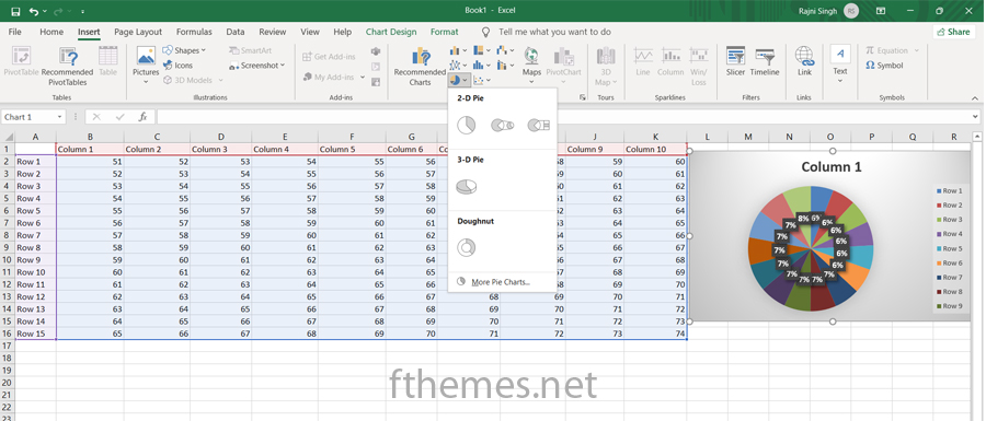
Step 2: Next, you need to choose the ‘3D Pie’ option.

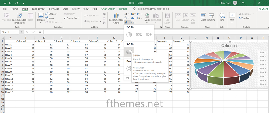
Step 3: After that just tap on the design option of your choice which will be displayed on the top of your screen. Choose any one you prefer!

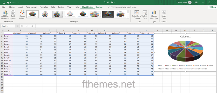
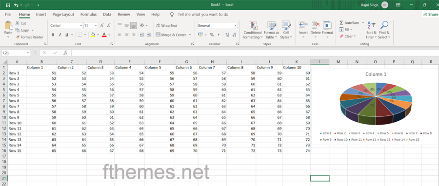
Step 4: You will notice that the above 3D style pie chart is now displayed on your spreadsheet.

Rotation of A Pie Chart in Excel

• To rotate your pie chart, double-click on the logo.
• Select the three-bar symbol under "Format Data Point".
• Then, change the "Angle of initial slice" until the pie chart is rotated to the desired degree. That's all there is to it!
• You're well on your way to producing clean, eye-catching pie charts for your marketing materials to emphasise crucial facts and compel stakeholders to act.

Excel Tips

Now that you know how to construct a pie chart in Excel, let's try to assemble a list of the most important do's and don'ts for making your pie graphs relevant and visually appealing.

• Sort the slices according to their size. Sort the slices from largest to smallest, or vice versa, to make estimating the pie chart percentages easier.
• Slices should be grouped. If a pie chart has several slices, divide them into meaningful pieces and use a different hue for each group and a different shade for each slice.
• Remove little pieces of grey: If your pie graph contains a lot of little slices (say, less than 2%), grey them out or add another" category.
• To bring smaller slices to the front of a pie chart, rotate it. Include only a few data categories. A pie chart with too many segments might become cluttered. If you have more than 7 data categories to plot, try utilising a pie of pie or bar of pie chart, and shift tiny categories to the secondary chart.
• Don't bother with a legend. Consider immediately identifying the pie chart slices so that your readers don't have to switch between the legend and the pie.
• Avoid using a lot of 3-D effects. Avoid applying too many 3-D effects in a single graphic since they might distort the message greatly.

Conclusion

The above article talks about the creation of pie charts in a spreadsheet which is another interesting function to learn about for organising data. Apart from learning about how to insert data in a pie chart and display it in the right manner, we have also shared some tips on using MS-Excel.

You can reach out to our HubSpot experts to troubleshoot any particular issue you’re facing or have a custom HubSpot development requirement. If you’re having short on resources to take care of the CMS Hub configuration and other day to day HubSpot tasks, check out our HubSpot CMS management service by FThemes.

Talk soon!