How to Alphabetize in Excel

In this article of how to Alphabetize in excel , you will learn how to set Excel in alphabetical order quickly and easily. It also offers answers to non-trivial jobs, such as how to alphabetize by the last name whenever the entries begin with the very first name.

In Excel, alphabetizing is as simple as ABC. Whether you're sorting a whole worksheet or a specific range, vertically (a column) or horizontally (a row), ascending (A to Z) or descending (Z to A), most tasks can be completed with a single click of a button. 

Nevertheless, in some cases, the constructed functions may fail, but you may still use formulas to sort by alphabetically.

This tutorial will teach you how to alphabetize your data in Excel by utilising the Sort and Filter capabilities to order it from A to Z. This function is especially beneficial for huge datasets when manually alphabetizing information in Excel would take a very long time. So you need to know how to Alphabetize in excel.

How to Alphabetize Columns in Excel

Follow the steps given below to Alphabetize multiple columns at the same time in Excel. 

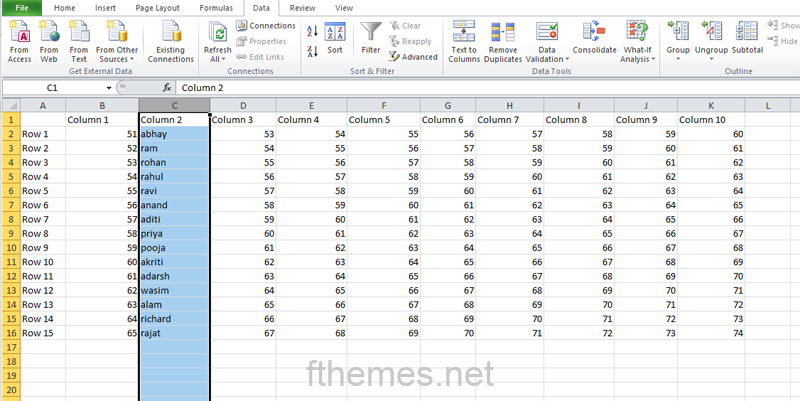
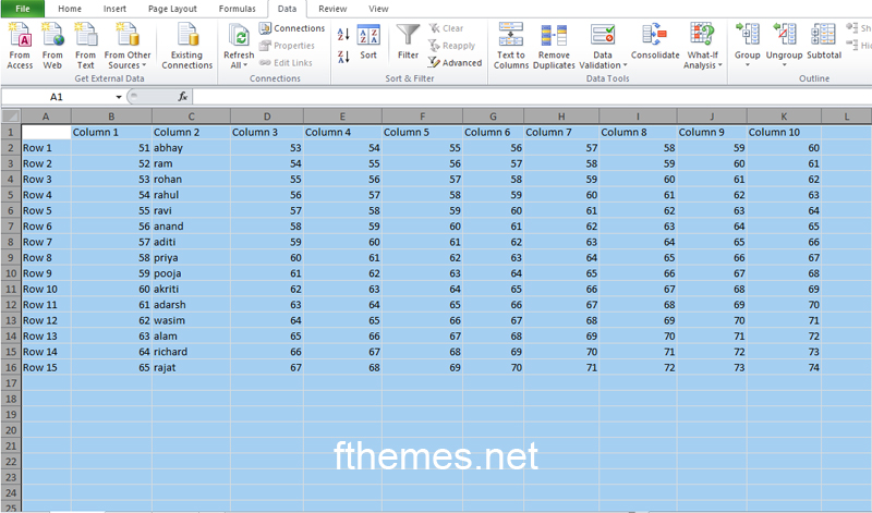
Step 1: First you need to select the table that needs to be Alphabetized.

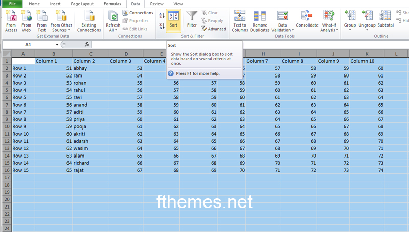
Step 2: Next you need to tap on the sort button on the Data tab. 

Step 3: After that, you will notice a ‘Sort’ dialogue box will appear on your screen on which you need to select the Column option from the drop-down menu and then select the column based on which you will Alphabetize your entire information.

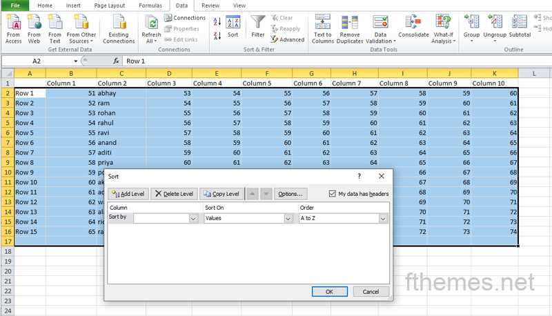
Step 4: Next in the ‘Sort On’ drop down you need to tap on the ‘Values’ option. If you use that option then you can also sort your entire data based on the cell colour or font colour of cell icons.

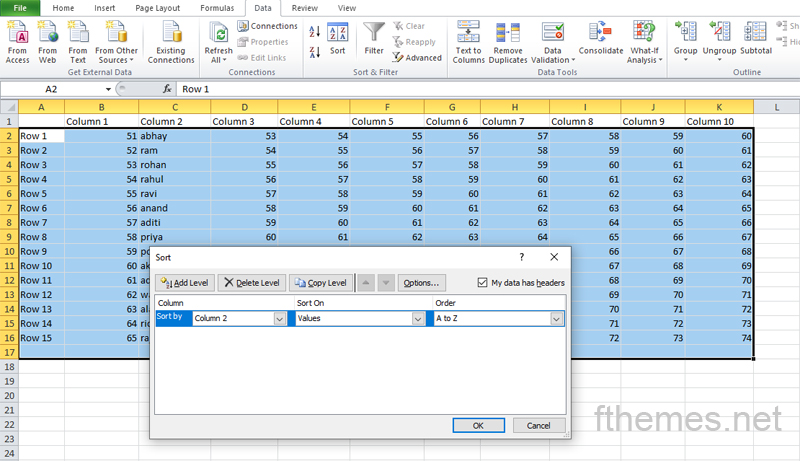
Step 5: In the next step, you need to select the ‘Order’ that is ‘A-Z’ for ascending and ‘Z-A’ for descending sort. In case your data is in the header row then just tap on uncheck in the option ‘My data has headers’ checkbox or just leave it checked.

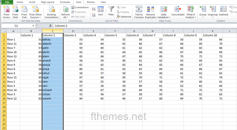
Step 6: Lastly, tap on the Ok button and your data or information has been sorted.

How to Alphabetize in Excel By Last Name

Microsoft Excel has a wide range of capabilities that allow it to handle a wide range of jobs. Many, but not all of them. If you're confronting a problem that doesn't have a built-in answer, chances are you can solve it using a formula. This holds true for alphabetical sorting as well.

Here are a handful of examples of when alphabetical order can only be accomplished via formulae. Because there are a few different ways to write names in English, you may occasionally find yourself in a position where the entries begin with the first name and you need to alphabetize them by the final name.

In this scenario, Excel's sort choices are ineffective, so let's turn to formulas.

Step 1: Insert the following formulae in two distinct cells with a complete name in A2, and then replicate them along with the columns to the last cell containing data:

Step 2: Extract the first name from C2:

=LEFT(A2,SEARCH(" ",A2)-1)

Pull the final name from D2:

=RIGHT(A2,LEN(A2)-SEARCH(" ",A2,1))

The components were then concatenated in reverse order, separated by a comma:

=D2&," "&C2"

Step 3: The formulae are explained in depth here, but for now, let's simply look at the results:

Step 4: Because we need to alphabetize the names rather than the formulae, turn them to values. To do this, select all of the formula cells (E2–E10) and copy them with Ctrl + C.

Step 5: Right-click the chosen cells, pick Values from the Paste Options menu, then press the Enter key:

Step 6: Good work, you're almost there! Select any cell in the resultant column, then click the A to Z or Z to A button on the Data tab to get a list alphabetized by the last name:

Step 7: If you need to go back to the old First Name Last Name format, you'll need to perform a bit of extra work:

Step 8: Split the names again into two halves using the following formulae (where E2 is a comma-separated name):

Obtain the first name:

=RIGHT(E2, LEN(E2) - SEARCH(" ", E2))

Get the last name:

=LEFT(E2, SEARCH(" ", E2) - 2)

And bring the two parts together:

=G2&" "&H2

Step 9: One more pass through the formulae to value conversion, and you're done!

Note: The method may appear complicated on paper, but it will only take a few minutes in Excel. It will take less time than studying this lesson, much alone manually alphabetizing the titles.

How to Alphabetize in Excel Keeping Rows Together

In one of the earlier instances, we explored utilising the Sort dialogue box to alphabetize rows in Excel. We were working with a correlated collection of data in that situation. But what if each row includes its own set of data? How do you alphabetize each row separately? If you have a reasonable number of rows, you can perform these procedures one by one to sort them but for that, you also need to know how to Alphabetize in excel. That would be a huge waste of time if you had hundreds or thousands of rows. Formulae may do the same task considerably more quickly.

Step 1: To start, copy the row names to another worksheet or another place on the same sheet, and then use the matrix formula below to alphabetize each row (where B2:D2 is the very first row in the tablespace):

=INDEX($B2:$D2, MATCH(COLUMNS($B2:B2), COUNTIF($B2:$D2, &$B2:$D2), 0))

Step 2: Please keep in mind that the right way to input an array formula in Excel is Ctrl + Shift + Enter.

Step 3: If you are unfamiliar with the Excel array formula, please follow these procedures to accurately input it in your worksheet:

• In the first cell, type the formula and hit Ctrl + Shift + Enter. Excel will surround the formula in curly brackets when you do this. Attempting to type the brackets manually will not work.
• To replicate the formula to other cells in the first row, select the formula cell and drag the fill handle to the right.
• To duplicate the formula to other rows, select all of the formula cells in the first row and drag the fill handle downwards.

Note: The method above works with two caveats: your source data should not contain any empty cells or duplicate values.

If your dataset has any blanks, use the IFERROR function to enclose the formula:

=IFERROR(INDEX($B2:$D2,MATCH(COLUMNS($B2:B2),COUNTIF($B2:$D2),0)), "")

Unfortunately, duplicates do not have a simple remedy.

How to Alphabetize a Column in Excel

Using Excel Ribbon Method:

Step 1: First you need to select the entire list that you wish to organise and sort in order.

Step 2: After that, you need to find the data tab on the excel ribbon and just tap on the A-Z icon to sort the order in ascending order and Z-A to sort the order in descending order.

Conclusion

You should go through the entire article if you wish to master all the above-mentioned skills in MS-Excel. It will not only help you arrange your data in order but also present your data at your workplace in an organised way. Just go through all these methods and learn excel concepts at your fingertips.

You can reach out to our HubSpot experts to troubleshoot any particular issue you’re facing or have a custom HubSpot development requirement. If you’re having short on resources to take care of the CMS Hub configuration and other day to day HubSpot tasks, check out our HubSpot CMS management service by FThemes.

Talk soon!